Name of Project:
Capturing chaos: a fast, stochastic, and scalable approach to Lorenz-96
Proposal in one sentence:
My group and I are building a fast and automated approach to chaotic dynamic systems and we want to test it on the Lorenz-96 problem.
Description of the project and what problem is it solving:
ABSTRACT / INTRODUCTION
Over the past decade, extreme weather events have increased and in the US there were $145 billion in damages and 688 deaths in 2021 alone [1]. The unpredictability of atmospheric phenomena is growing. Weather is regarded as a chaotic system because the smallest of errors in forecasting spiral into much larger errors over time. This is a major challenge for weather forecasting and we believe our group is in a good position to tackle it in a new and potentially better way. We have compared our methods to two common neural net based techniques used in dynamic systems modeling: long short-term memory (LSTM) and gated recurrent unit (GRU), using an experimental dynamic system, ‘Casaded Tanks’, as a benchmark. We saw that our results were more accurate and took a fraction of the time to compute. [3] In our preliminary testing we have also seen that we have performed promisingly compared with SINDy, a state-of-the-art method for modeling chaotic dynamic systems. This grant will enable us to focus on chaotic systems, starting with the Lorenz-96 model. Edward Lorenz formulated a relatively simple model of a chaotic system in his seminal 1996 paper [2]. Since then, the model has become a benchmark, tackled by many deterministic machine learning methods. Our group seeks to provide a solution by utilizing a Bayesian approach in a Gaussian Process (GP). The GP we use is faster and potentially more accurate for dynamic systems because it implements a Karhunen-Loève expansion. Our plan is to further compare our method to SINDy and other neural net approaches such as reservoir computing techniques on Lorentz-96 and other chaotic system benchmarks.
BSS-ANOVA and KL DECOMPOSED GPs
Our group has developed a less common type of Gaussian Process which is gaining attention recently [4]. Unlike other GPs our method utilizes a Karhunen-Loève expansion, more specifically a decomposed kernel BSS-ANOVA. The BSS-ANOVA is O(NP) in training and O(P) per point in inference where P is the number of terms included after truncation of the ANOVA/KL expansion and N is the size of the dataset. We have created a new type of Bayesian optimizer which quickly and effectively builds and trains the model, ensuring that P<<N. Because of its speed and accuracy combination for small-to-moderate feature space dimension sizes it is possible to model the derivative information in a dynamic system as a static problem, then to integrate the learned dynamic model given initial conditions and forcing function inputs to make predictions. This means it needs much less data to train accurately than a recurrent neural network, which learns patterns in the training data and makes predictions through those learned patterns.
PRELIMINARY TESTING
When comparing our method to recurrent and deep learning neural networks we have seen more accurate results and faster computation time on a pair of dynamic system benchmarks. In a recent publication we compared our method to neural nets and some other methods for static prediction on the experimental Cascaded Tanks benchmark and a specially designed SIR synthetic benchmark [3].
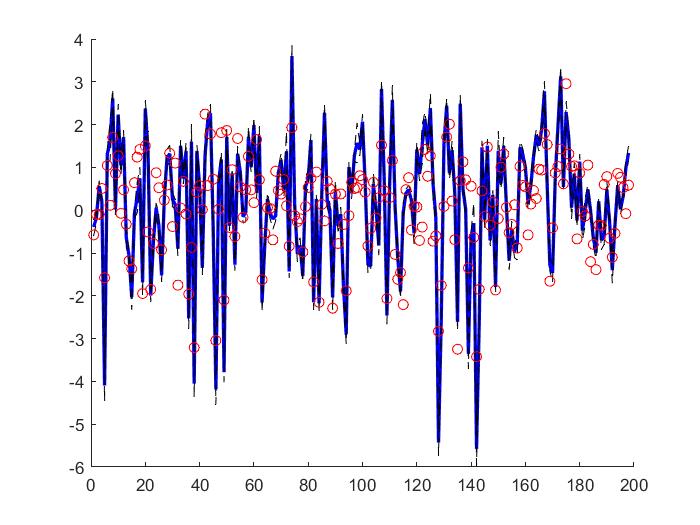
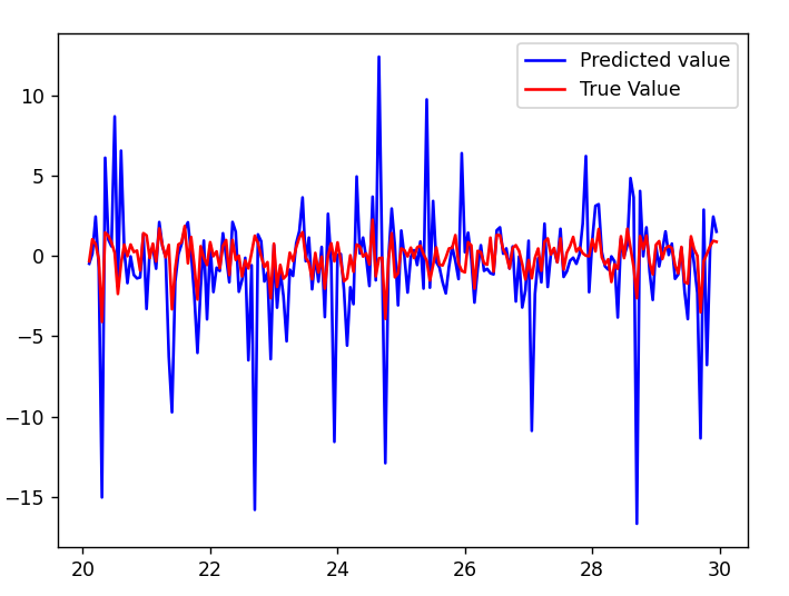
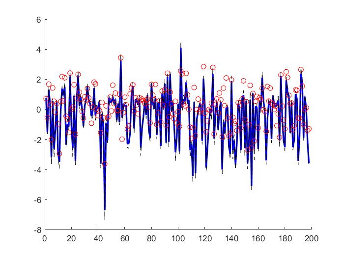
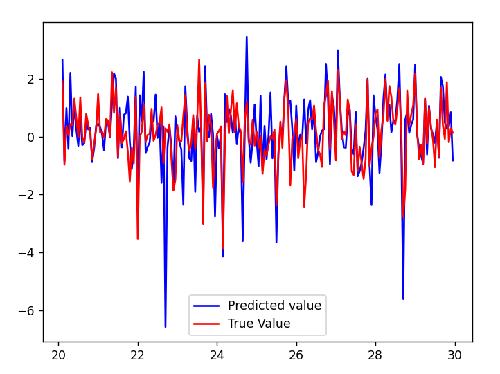
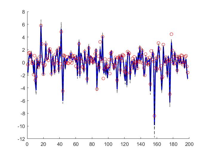
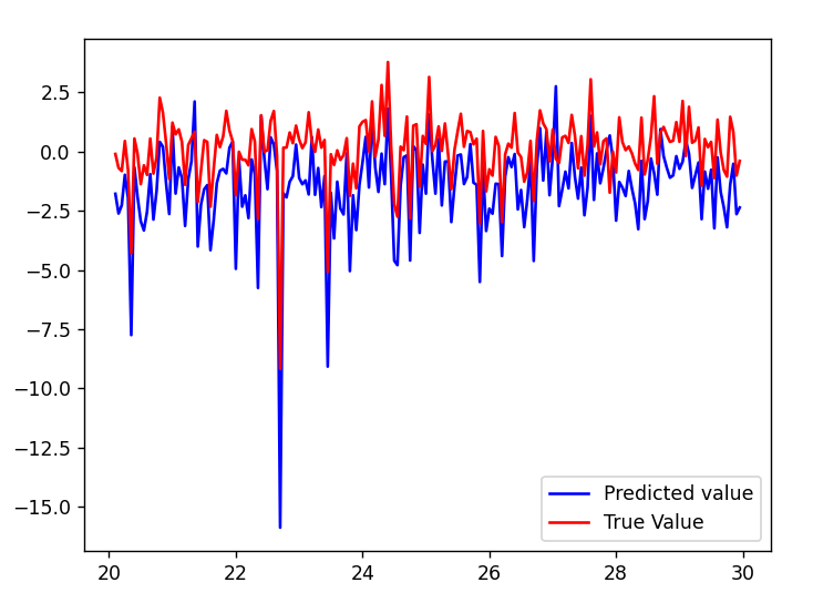
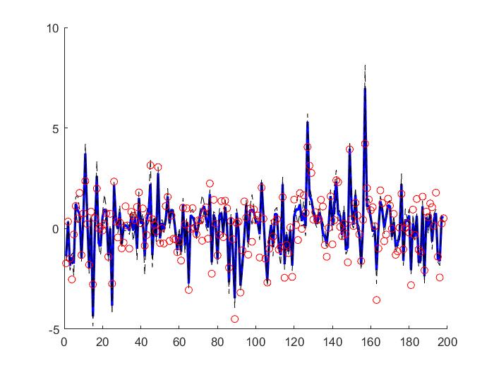
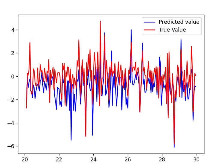
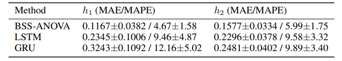
The Cascaded Tanks problem is an experimental nonlinear dynamic system benchmark. In this problem there are two tanks and a reservoir. The upper tank is filled with water from the reservoir by a pump. A signal is sent to the pump to control the inflow of the water. A drain connects the upper tank with a lower tank, which in turn drains back into the reservoir. This system is moderately nonlinear in theory. In the static derivative estimation problem we compared with a residual deep network and a random forest, which we bested in accuracy as shown in Table-1. For dynamic prediction we compared our method to two neural networks: an LSTM and a GRU. Our method – which is not parallelized or optimized for speed – took an average of 20.22 seconds. The neural networks took an average of 175 seconds and 123 seconds, respectively. The results can be seen in Figure-1 and Table-2.
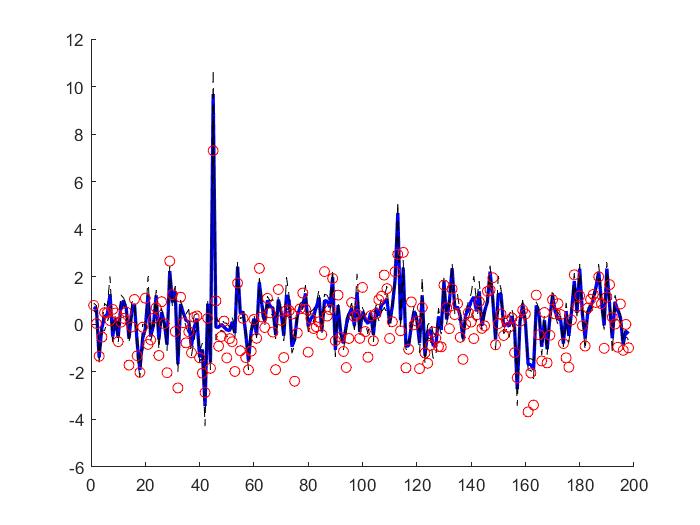
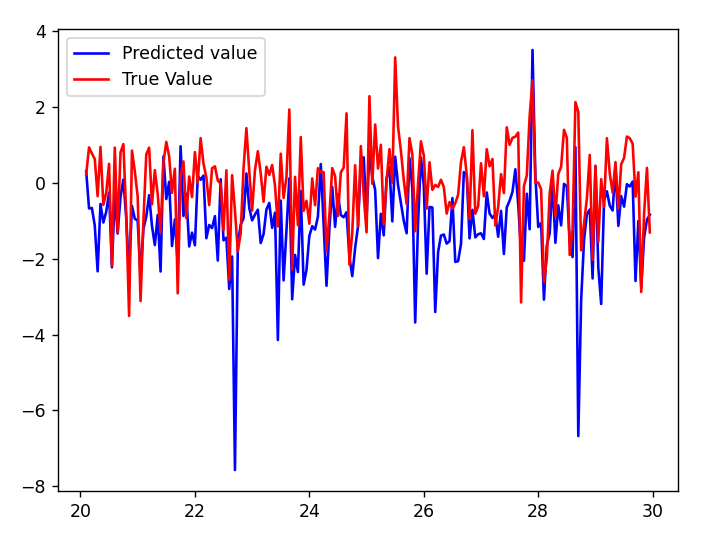
Additionally we tested both methods against a synthetic nonlinear benchmark dataset based on the nonlinear ‘Susceptible, Infected, Recovered’ system, in which the infectiousness parameter was used as a forcing function. The training set consisted of only constant values of infectiousness, while the test set contained varying functions. The GP was able to accurately replicate the training set behavior while the neural networks were not.
Figure 1: (a) LSTM and (b) our method predictions vs test data for the height of the water in the tank 1 in the Cascaded Tanks problem. Shaded region represents 95% confidence.
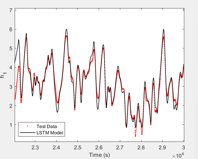
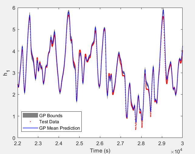
Table 1: Cascaded tanks 5-fold cross validated accuracies: derivatives [3]
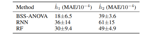
Table 2: Cascaded tanks 5-fold cross validated accuracies: timeseries [3]
DISCUSSION/FUTURE WORK
After completing this grant, we will look to expand our scope of benchmark problems, while starting with outreach to organizations who might stand to benefit from faster and more accurate tools for modeling chaotic systems. Computational Fluid Dynamics (CFD) models are a general class of chaotic systems we wish to model in the future. The market for accurately modeling CFD is valued to be over $2 billion [5]. This is because the application of CFD incompacess a wide array of topics. Just to name a couple: aerodynamics of a car and heat transfer of pipes. Chemical reaction networks (CRN) is another potential future research area. CRN models the behavior of chemical reactions and are also sometimes chaotic in nature.
RESEARCH SCHEDULE
Week 1: Utilize high-performance computing cluster to create high-resolution data points from the Lorenz-96 model
Week 2-4: Build and test models
Week 5-6: Extension to other models and the building of a public repository
Grant Deliverables:
- High resolution lorenz-96 datasets
- Model of Lorenz-96 created from our routines
Squad
Dr. Dave (Research Advisor): Discord doktordave#4611
Kyle (Graduate Researcher): Discord Kyle Hayes#9643
Josh (Undergraduate Researcher): Discord NASAbanyo#3464
Charlie (Undergraduate Researcher): Discord Pinhead#4590
References
[1] NOAA. 2021 U.S. billion-dollar weather and climate disasters in historical context. Accessed at: 2021 U.S. billion-dollar weather and climate disasters in historical context | NOAA Climate.gov
[2] E.N. Lorenz. Predictability: A Problem Partly Solved. Accessed at: Predictability: a problem partly solved | ECMWF
[3] D.S. Mebane et al. Fast variable selection makes scalable Gaussian process BSS-ANOVA a speedy and accurate choice for tabular and time series regression. Accessed at: [2205.13676v1] Fast variable selection makes scalable Gaussian process BSS-ANOVA a speedy and accurate choice for tabular and time series regression
[4] P Greengard et al. Efficient reduced-rank methods for Gaussian processes with eigenfunction expansions. Accessed at: https://arxiv.org/abs/2108.05924
[5] Computational Fluid Dynamics Market: Global Industry Trends, share, size, growth, opportunity and forecast 2022-2027. Accessed at: Computational Fluid Dynamics (CFD) Market | Share, Size, Trends, Industry Analysis and Forecast 2022-2027.